-
Introduction
We have started this page in an attempt to give users guidance on how to read ACOS data in different software packages. We prepared relatively simple examples in IDL and Python, and hope to add MatLab soon. To remind, ACOS data are in HDF5 format.
The emphasis here as given on reading and quality screening is done on purpose. These steps are the most important to understand by novice users. Once they become confident in opening files and reading data from there, they can augment examples here with the particular usage they have in mind.
-
IDL
-
Basic reading example
The following section describes the most basic steps needed to open and read one science data field, in particular the xCO2 retrieval (total column CO2 dry-air molar-mixing ratio), from an ACOS Level 2 file, from a collection we name "ACOS_L2S". Full collection and sample files can be acquired from our archive at:
http://oco2.gesdisc.eosdis.nasa.gov/data/
or, from Mirador.
In this example, we open an ACOS HDF5 file, open interface to science data field that contains the data "/RetrievalResults/xco2", check its size, and if larger than 0 bytes proceed to read the data, and close the open interfaces to the data field and the file. Because of the "IF..." statement that spawns for more than one line, we have to be careful how this code is executed. Save this snippet in a text file, say, "foo.pro", and execute within IDL (in the IDL command line) as:
.rnew foo.pro
file_name="file_name_of_downloaded_ACOS_file.h5"
f_id=H5F_OPEN(file_name)
co2_id=H5D_OPEN(f_id,"/RetrievalResults/xco2")
sz=H5D_GET_STORAGE_SIZE(co2_id)
IF(sz GT 0) THEN BEGIN
xco2= H5D_READ(co2_id)
ENDIF ELSE BEGIN
print,"Null-size data. Skip to the next file"
ENDELSE
H5D_CLOSE,co2_id
H5F_CLOSE,f_id
END
-
Advanced example: Reading multiple data fields, from multiple files; Quality screening; Multi-day aggregation and gridding of ACOS Level 2 data.
This example is a bit more advanced. It adds to the above basic steps a multi-datasets and multi-file reading, augmenting data in a vector arrays in memory, quality screening, gridding to a 2x2 degree cylindrical map, and plotting. Apart from the quality screening, all of these are examples of optional functions and procedures that can be used in IDL.
NOTE: The quality screening in this IDL program, using the "/RetrievalResults/master_quality_flag", is ONLY applied to v2.9. (Download the program; Execute in IDL as .rnew AcosL2Binner). For scientific analysis on ACOS data, please follow the science team's recommendation from User's Guide.
Upon successful run on two different 60-day periods, in Boreal winter and summer in 2010, and using only "Good" and "Caution" quality, the following plots can be produced, for data from V2.9 algorithm builds:

The March-April time in the Northern Hemisphere is just at the onset of the vigorous spring biomass growth. Hence, the CO2 amounts in the atmosphere reflect the accumulated over the winter seasonal peak. Correspondingly, early in the fall, by September-October, the photosynthetic activity removed and stored in the annual biomass (foliage, grass, crops, etc.) respective amounts of CO2, bringing the concentrations to their seasonal minimum.
Note: All IDL examples are using functionality that comes with the standard IDL distribution. No additional libraries or modules are required.
-
-
Python
-
Basic Reading Example.
In this section we describe how to open and read an ACOS science data field using python, in a manner similar to that of the IDL example above.
We will read the familiar "xco2" variable, from an ACOS Level 2 file archived at:
http://oco2.gesdisc.eosdis.nasa.gov/data/
To read the "xco2" variable, given node definition, variable name, and file name, we can use following script
Vars = {} #Init dictionary
node_name = "/RetrievalResults" #Node definition
v_n = "xco2" #Variable name
# Assign to dictionary
Vars['xco2'] = retrieve_hdf5_var(input_fileh5, v_n, node_name)
where retrieve_hdf5_var function defined as
def retrieve_hdf5_var(input_fileh5, v_n, node_name):
h5file = tb.openFile(input_fileh5, "r")
hdf5_object = h5file.getNode(node_name, v_n)
array = hdf5_object.read()
h5file.close()
return array
To be able to use the above functions, python module requirements are as follows:
python 2.7, numpy, and tables module
You can import them using following lines:
import numpy as np
import tables as tb # From pytables
-
Advanced Example: Similar to the IDL advanced example, we write a python script that reads multi h5 files, grid them (2x2 degree) using filtering options.
Code for python script can be downloaded from here. An example plot is also created below.

Plot in the left is created in Robinson projection from average of the 2 months of data (March, April-2010). Data can be downloded from
http://oco2.gesdisc.eosdis.nasa.gov/data/
While the simplest way to see and acquire the ACOS data files content through OPeNDAP is to use a browser (where the html url is a link to a data file:
http://oco2.gesdisc.eosdis.nasa.gov/data/
python gives the freedom and the power of scripting the data acquisition through OPeNDAP. The example below is using pydap module:
# The url below is just an example. Make sure to enter valid full OPeNDAP path to a granule from http://oco2.gesdisc.eosdis.nasa.gov/opendap/
import pydap.client
url = 'http://oco2.gesdisc.eosdis.nasa.gov/opendap/OCO2_L2_Standard.7/2016/018/oco2_L2StdND_08230a_160118_B7200_160119155905.h5'
dataset = pydap.client.open_url(url)
# to see the list of variables
dataset.keys()
# to open one of the variable
myarray = dataset['sounding_altitude']
Additionally it should be noted that, there are multiple choices for reading file from OPENDAP using python. To see other options search Google and find pages similar to https://publicwiki.deltares.nl/display/OET/Reading+data+from+OpenDAP+using+python. -
-
MATLAB
-
Basic reading example
This is a simple code to read an ACOS data file with matlab and is simillar to IDL as shown above.
Here the program reads xco2 correspond to respective geolocation latitudes and logitudes and also get
the information regarding the attributes such as unit and missing value.i FILE_NAME='acos_L2s_090405_41_Production_v050050_L2s20900_r01_PolB_111017194653.h5'
file_id = H5F.open (FILE_NAME, 'H5F_ACC_RDONLY', 'H5P_DEFAULT');
DATAFIELD_NAME = 'RetrievalResults/xco2';
data_id = H5D.open (file_id, DATAFIELD_NAME);
Lat_NAME='SoundingGeometry/sounding_latitude_geoid';
lat_id=H5D.open(file_id, Lat_NAME);
Lon_NAME='SoundingGeometry/sounding_longitude_geoid';
lon_id=H5D.open(file_id, Lon_NAME);
xco2=H5D.read (data_id,'H5T_NATIVE_DOUBLE', 'H5S_ALL', 'H5S_ALL', 'H5P_DEFAULT');
lat=H5D.read(lat_id,'H5T_NATIVE_DOUBLE', 'H5S_ALL', 'H5S_ALL', 'H5P_DEFAULT');
lon=H5D.read(lon_id,'H5T_NATIVE_DOUBLE', 'H5S_ALL', 'H5S_ALL', 'H5P_DEFAULT');
ATTRIBUTE = 'Units';
attr_id = H5A.open_name (data_id, ATTRIBUTE);
units = H5A.read(attr_id, 'H5ML_DEFAULT');
H5A.close (attr_id);
H5D.close (data_id);
H5D.close (lat_id);
H5D.close (lon_id);
H5F.close (file_id);
afiledata=[lat lon xco2]
Note: This works with matlab version 7.1 or higher with appropriate library. Data can be saved in mat format as save('filename', 'var1', 'var2', 'var3') or in ascii as save('filename', 'var1', 'var2',.., '-ascii'). By default, MAT-files are double-precision, binary files. For getting higher precision add 'format short eng'. -
Advanced Example: Similar to the IDL advanced example, we write a MATLAB script that reads multi h5 files, grid them (2x2 degree) using filtering options.
Code for MATLAB script (version. R2009a) can be downloaded from here.
Note: For the purpose of viewing the gridded products on a map, we recommend to use Panoply as a data viewer tool. However, to be plotted by Panoply, dataset variables must be tagged with metadata information using a convention such as CF. We use the MATLAB script above to save the variable in a simple netCDF CF-compliance. The script is following:
% Now we try to make the data output to netCDF-CF1 compliance file
% viewing tools, such as Panoply, can easily view the results
%%%%%%%%%%%%%%%%%%%
% Initialize a file
%%%%%%%%%%%%%%%%%%%
ncid = netcdf.create('foo.nc','nc_write');
% Define dimensions: latdimID = netcdf.defDim(ncid, 'latitude',Ny);
londimID = netcdf.defDim(ncid, 'longitude',Nx);
% Define axis:
Y = -89:2:89; %latitude grids
X = -179:2:179; %longitude grids
latID = netcdf.defVar(ncid,'latitude','float',latdimID);
lonID = netcdf.defVar(ncid, 'longitude','float',londimID);
varID = netcdf.defVar(ncid, 'avg_xCO2','float',[londimID, latdimID]);
% Write the variable to nc file
%varname = 'avg_xCO2';
%long_name = 'gridded average of CO2 in ppm';
%unit = 'ppm';
% Put attributes:
netcdf.putAtt(ncid, latID,'units', 'degrees_north'); % This units requires for Panoply to recognize the dimension
netcdf.putAtt(ncid, lonID,'units', 'degrees_east'); % as well as this units
netcdf.putAtt(ncid, varID,'units', 'ppm');
netcdf.putAtt(ncid, varID, '_FillValue', nanfill);
netcdf.endDef(ncid);
netcdf.putVar(ncid, varID, co2_grid);
netcdf.putVar(ncid, latID, Y);
netcdf.putVar(ncid, lonID, X);
% We can now close the cdf file (optional):
netcdf.close(ncid)
You can see the figure from Panoply in the following (the same plot generated by IDL is shown in the IDL_advanced):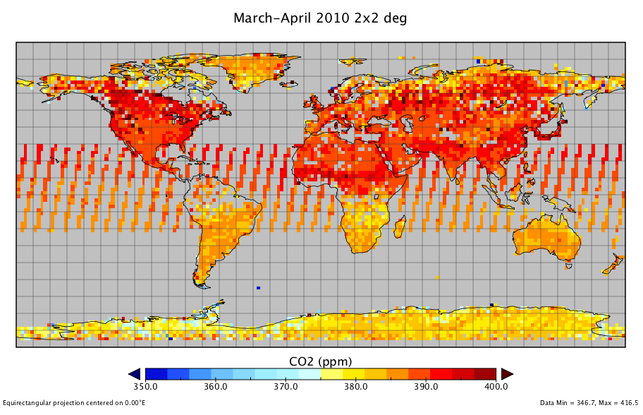
-